PIV Theory
PIV is a non-intrusive laser diagnostic capable of determining instantaneous two-dimensional velocity fields corresponding to the cross-sectional slices of three-dimensional flows. The operating principle of PIV stems from the following simple relation: \( \overline{V}={\Delta \overline{X}}/{\Delta t} \). That is, average velocity, \( \overline{V} \), is equal to the displacement, \( \Delta \overline{X} \), divided by the change in time, \( \Delta t \).
In practice, the exploitation of this equation starts with the seeding of a flow with particles capable of scattering laser light. However, the seeding particles must also be able to attain velocity equilibrium with the fluid flow, i.e., particles must follow the flow with minimal response time, \( {\tau }_s \). That is, if the response time of a seeding particle is small, then the velocity of the seeding particle will mirror that of the surrounding fluid flow with high fidelity. Equation 1 shows that \( {\tau }_s \) is a function of particle diameter, \( d_p \), particle density, \( {\rho }_p \), and dynamic viscosity of fluid, \( \mu \).
\( {\tau }_s=d^2_p\frac{{\rho }_p}{18\mu } \) (1)
It is obvious that small particles will follow fluid flow better than large particles of equal density will, but care must be taken when selecting seeding particles, as larger particles, in general, scatter more light.
Once a flow has been properly seeded (see Fig. 1), the laser sheet can be used to illuminate a two-dimensional slice of the flow. That is, as a laser sheet slices through the particle-seeded flow, the seeding particles scatter the light in all directions. Note that particle scattering characteristics are a function of laser power, wavelength, and polarization, as well as a function of particle size and shape, refractive index ratio, and detection angle. It is also important to stress that laser power and seeding density are important factors in achieving high-fidelity data, as the scattering observed during PIV measurements typically falls within the Mie scattering regime. Namely, Mie scattering, as opposed to Rayleigh scattering, is usually present during PIV measurements, as the effective diameters of scattering particles are typically much greater than the excitation wavelength, i.e., \( d_p\mathrm{>}\mathrm{>}{\lambda }_L \). In this scattering regime, side scattering, i.e., scattering in the direction normal to the laser sheet, is substantially less than forward scattering, making it challenging to collect sufficient signal when imaging the side scattering.
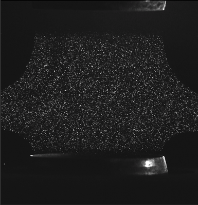
Figure 1. Sample image of scattering seeding particles.
Regarding \( \overline{V}={\Delta \overline{X}}/{\Delta t} \), particle displacement is determined by imaging scattered light from two sequential laser pulses, i.e., image frames F1 and F2, that are separated in time by . The field of view imaged by the camera is divided into interrogation areas (IAs), and the IA of F1 are adaptively correlated with those of F2. Unlike the traditional cross-correlation method in which IAs are fixed in size and shape, the adaptive method utilizes IAs whose size and shape change iteratively. That is, adaptive IAs will change to better accommodate differences in local seeding densities and velocity gradients. In the comparison of F1 and F2, signal peaks corresponding to individual scattering particle are identified, and the resulting displacement, \( \Delta \overline{X} \), is then calculated. Since the time between laser pulses is user-defined, velocity vectors can consequently be determined. A visual representation of the PIV process is depicted in Fig. 2. When performing adaptive PIV in DantecStudio, input settings must be specified on the following four tabs: Interrogation areas, Window/Filter, Validation, and Adaptivity. All settings are summarized in Table 1 by tab name.
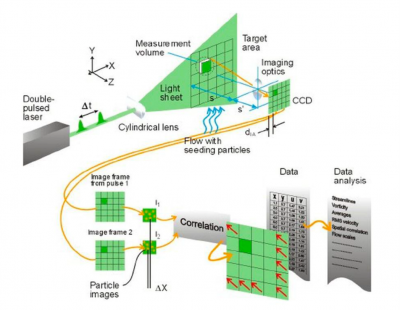
Figure 2. Visual representation of PIV data collection and processing methodologies. Figure adapted from DantecStudio User’s Guide. Dantec Dynamics,
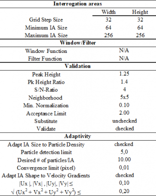
Table 1. DantecStudio input settings for Adaptive PIV.
The uncertainty of PIV measurements was quantified by analyzing the full-scale accuracy and resolution uncertainties of the measurements. The full-scale accuracy of PIV measurements is represented by:
\( FSA={\left[{\left({{\sigma }_t}/{T}\right)}^2+{\left({{\sigma }_d}/{D}\right)}^2\right]}^{1/2} \) (2)
where \( {\sigma }_t \) and \( {\sigma }_d \) are the discriminative minimum period between laser pulses and displacement, respectively, and and are the time between laser pulses and the maximum displacement (as per the quarter rule), respectively. Since the discriminative minimum period between laser pulses is typically much less than the time between laser pulses for Nd:YAG lasers, i.e., \( {\sigma }_t\ll T \), the first term in Eq. 2 can be disregarded, leaving \( \ FSA={{\sigma }_d}/{D} \). The discriminative displacement is defined as pixels. The maximum displacement was set at \( D=16 \) pixels, or ¼ of the height and width of an IA comprised of 64×64 pixels. Note that since adaptive PIV methods are used here, not all IAs were of the same size. However, since the majority of IAs contained 64×64 pixels, this IA size is adopted for determining the maximum displacement. The resulting full-scale accuracy is found to be 0.625% of the maximum displacement.
The uncertainty due to the full-scale accuracy of the PIV measurements is combined with that due to image resolution uncertainty. That is, the image resolution is determined to be 131±2 pixels/mm for all PIV measurements, and the uncertainty in image resolution propagated into the uncertainty of PIV measurements, as the image resolution is used to calibrate particle displacement readings (pixels per image pair). Linear error propagation analysis is used to quantify the effect of image resolution on velocity uncertainty. The total uncertainty of PIV measurements on a vector-by-vector basis is then calculated as the root sum square of the FSA- and resolution-induced uncertainties. A convergence study is also performed to determine the number of image pairs required to achieve convergence of velocity values.
PIV Experiment
Here, PIV measurements are performed using a Litron Nano (L200-15PIV) laser that outputted 532 nm beams at a repetition rate of 12 Hz and a pulse energy of 200 mJ. Scattered light is collected by an AF Micro-Nikkor 200 mm lens (f/16) and then imaged using a Dantec Dynamics FlowSense 4M MKII camera (12-bit CCD), which is equipped with a bandpass filter that had a central wavelength of 532 nm; the QE of the camera is approximately 55% at 532 nm. Figure 3 depicts a schematic of the PIV experimental setup.
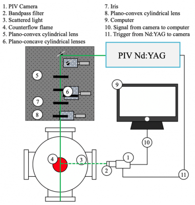
Figure 3. Schematic of PIV experimental setup.
For the counterflow non-premixed flame demonstrated here, medical nebulizers (Sunrise Medical HHG Inc.) are a cost-effective means of generating seeding droplets. Both the fuel and oxidizer streams are equipped with a nebulizer that is filled with silicone oil (50 cSt). During PIV tests, flow is directed through these nebulizers to atomize the silicone oil, resulting in micron-sized spherical droplets. The flow rates through the fuel stream and oxidizer stream nebulizers are maintained at 2 and ≥3 L/min, respectively. Although the varying flow rates through the two nebulizers inevitably result in differences in seeding density between the fuel and oxidizer streams, the discrepancy in seeding density is regarded as a non-issue because adaptive PIV accounted for local seeding density when assigning IA size. However, if PIV vectors are generated using IAs of fixed size, then the differences in seeding density could be problematic. To best guarantee the convergence of velocity values, a minimum of 180 image pairs are collected during each test.
Although the nebulizers provided an inexpensive, easy to control means of generating seeding particles, unlike alumina oxide (Al2O3), silicone oil has a boiling point (570 K) that is well below flame-relevant temperatures. Thus, silicone oil droplets are unable to resolve the velocity field near the reaction zone of a counterflow flame, whereas alumina oxide particles would be able to resolve the velocity field in these high-temperature regions. Figure 4 illustrates how seeding density changes as the silicone droplets approach the flame. Even if alumina oxide were used instead of silicone oil, however, accurately resolving the velocity field in the high-temperature region of a counterflow flame is complicated by thermophoretic effects, which can cause the velocity of seeding particles to deviate from that of the surrounding flow field. Furthermore, solid seeding particles, such as alumina oxide, have a tendency to clog burners, potentially modifying the flow.
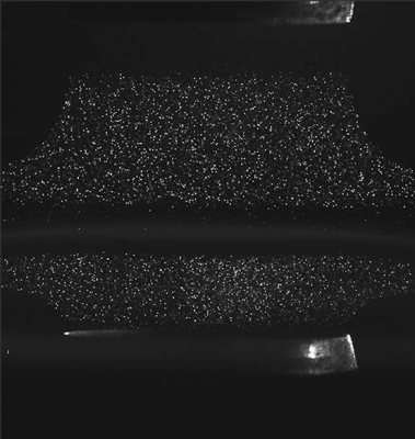
Figure 4. Sample image of silicone droplets during reacting PIV.
Figures 5 and 6 depict typical PIV seeding densities with the corresponding local velocity vectors for reacting and non-reacting cases, respectively. These figures are to illustrate a) the density of vectors after data processing, and b) how the silicone droplets evaporate as they approach the flame front. Note that the flame-like shape shown in Fig. 5 is a result of chemiluminescence imaged through a 532 nm bandpass filter, and is not necessarily representative of the actual flame. Although velocity vectors corresponding to the fuel and oxidizer streams are separated in Fig. 5 by a vector-less gap, this gap was created through the intentional removal of high-uncertainty velocity vectors. That is, since the DantecStudio software outputted vectors for all axial heights within the specified region of interest, even for those where seeding density is negligible, a systematic method is required to isolate the artificial, high-uncertainty velocity vectors. Although these bad vectors are easily identified based on their magnitude and direction, a convergence study is utilized to confirm the axial height range in which velocity vectors are invalid.
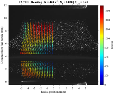
Figure 5. Sample reacting PIV results.
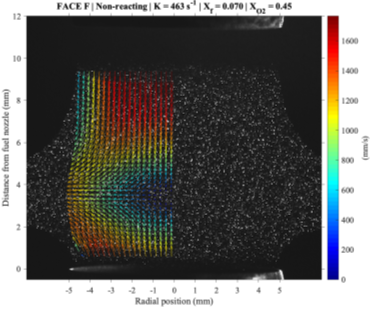
Figure 6. Sample non-reacting PIV results.